Cassandra: Mighty Storage Engine

Cassandra is built for speed: It can handle millions of writes per second with sub millisecond latency, and scales effortlessly across data centers.

And yes, that’s not just marketing pitch, those numbers are real. Some of the world’s biggest companies use Cassandra to crunch trillions of rows and petabytes of data, helping machines get smarter and making everyday life easier in the process.

Of course, reaching that kind of scale takes more than just good hardware. It requires a state of the art storage engine and clever data retrieval mechanics working behind the scenes.

If you’re new to Cassandra, feel free to check out the earlier posts in this series to get up to speed on how it all works.

• Cassandra: Write Fast, Scale Forever
• Cassandra: Internals & Architecture

Let’s explore the sophisticated and complex data storage layer of the Cassandra database.

Storage Engine

The storage engine is the part of a database that handles how data is saved, read, and organized behind the scenes. Think of it as the machinery under the hood deciding how data is written to disk, how updates and deletes are handled, how indexes are stored, and how the system recovers after a crash. Some engines are built for lightning-fast writes, while others are tuned for ultra-efficient reads.

The Cassandra storage engine is built for a world where uptime matters, data volumes are huge, and failures are expected.

Instead of rewriting data constantly, Cassandra takes a smarter, more resilient approach. It logs incoming data, holds it in memory temporarily, and writes it to disk in a way that favors fast appends and efficient reads. Over time, background processes clean up and reorganize the data to keep things tidy and performant.

Cassandra’s Storage Engine

Under the hood, a set of tightly integrated components: from memtables and SSTables to compaction and bloom filters work together to make this seamless.

Component	Region	Goal
Commit Log	Disk	Stores every write operation for durability and crash recovery
Memtable	Memory	Holds recent writes in-memory before flushing to disk
SSTable	Disk	Immutable, sorted files where data is persisted
Bloom Filter	Memory	Quickly checks whether a key might exist in an SSTable
Indexes	Memory + Disk	Helps locate data positions inside SSTables
Compaction	Background Process	Merges SSTables, clears tombstones, and improves read efficiency
Tombstones	Metadata	Mark deleted data so it can be removed during compaction

The components above hold a special place in the field of computer science. Each backed by decades of research, dedicated academic papers, and even entire books that dive deep into their logical foundations, design trade-offs, and mathematical underpinnings.

Commit Log

One of Cassandra’s core promises is durability.

Once it says a write is successful, that data is going to stick around, even if the system crashes. Just like other databases that care about durability, Cassandra does this by writing the data to disk before confirming the write. This write-ahead file is called the CommitLog.

Here’s how it works: every write hitting a node is first recorded by org.apache.cassandra.db.commitlog.CommitLog, along with some metadata, into the CommitLog file. This ensures that if something goes wrong, say the node crashes before the data hits memory or disk then Cassandra can replay the log and recover what was lost.

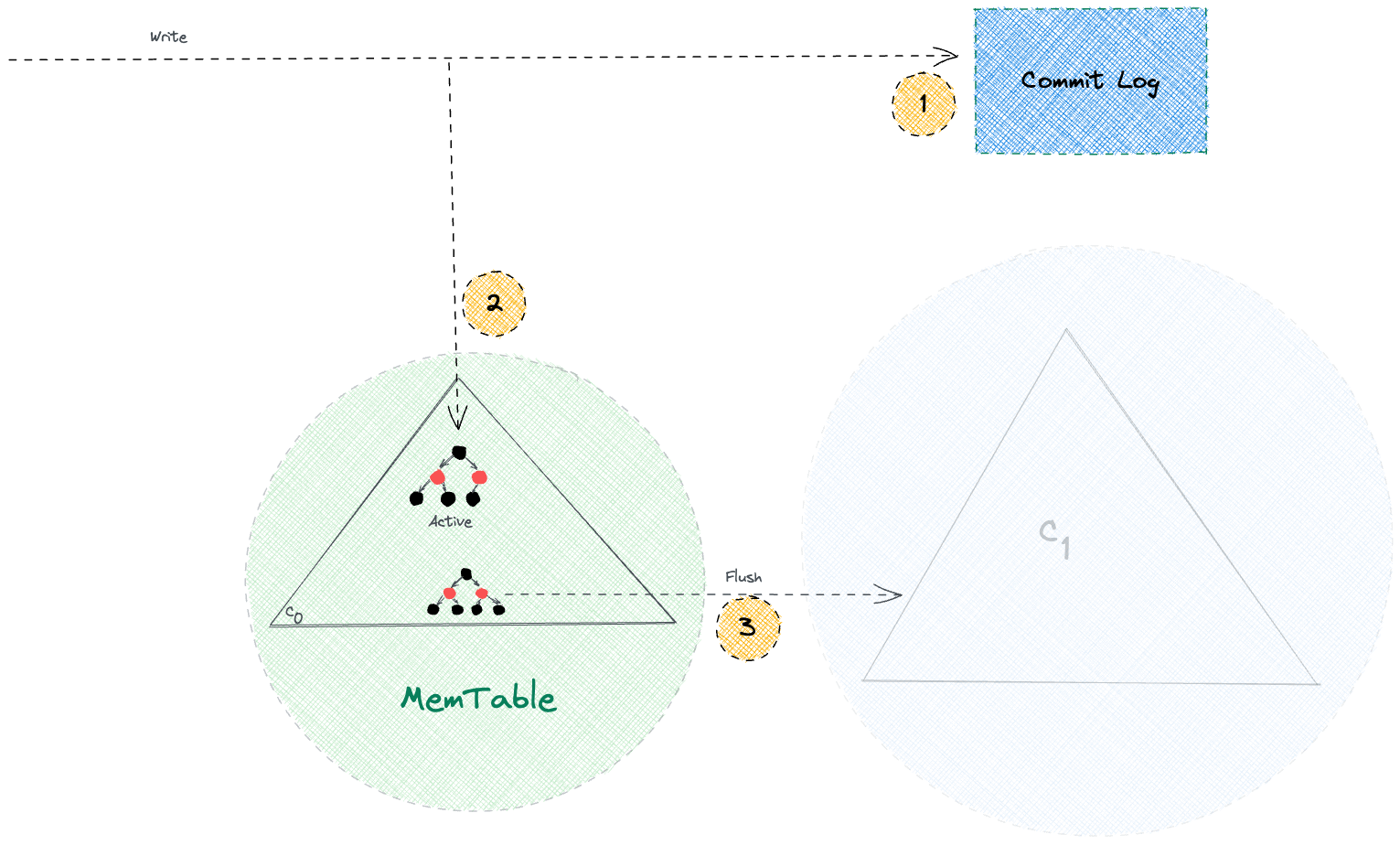
The CommitLog, MemTable, and SSTable are all part of the same flow. A write first goes to the CommitLog, then it updates the MemTable (an in-memory structure), and eventually, when certain thresholds are met, the MemTable is flushed to disk as an immutable SSTable. Once that happens, the related entries in the CommitLog are no longer needed and get cleared out.

When a node crashes, be it a hardware failure or an abrupt shutdown, Cassandra leans on the CommitLog to get things back in shape. Here’s how the recovery plays out:

• Cassandra starts reading CommitLog segments from the oldest one first, based on timestamps.
• It checks SSTable metadata to figure out the lowest ReplayPosition—basically, the point up to which data is already safe on disk.
• For each log entry, if it hasn’t been persisted yet (i.e., its position is beyond the known ReplayPosition), Cassandra replays that entry for the corresponding table.
• Once all the necessary entries are replayed, it force-flushes the in-memory tables (MemTables) to disk and recycles the old CommitLog segments.

This replay logic ensures no data is lost, even when things go sideways.

Memtables

MemTable is where Cassandra keeps recent writes in memory before they hit disk.

Think of it as a write-back cache for a specific table. Every write that comes in goes to the MemTable after it’s safely recorded in the CommitLog. Unlike CommitLog, which is append-only and doesn’t care about duplicates, MemTable maintains the latest state. If a write comes in for an existing key, it simply overwrites the old one.

Internally, it’s sorted by the row key, which makes reads faster for keys already in memory. It’s also why range queries perform reasonably well when the data is still in MemTable. But since it’s all in-memory, there’s always a limit. Once it grows past a certain threshold (based on size, time, or number of writes), Cassandra flushes it to disk in the form of an immutable SSTable and clears the MemTable.

So in essence, MemTable sits right between the volatile CommitLog and the durable SSTables, acting like a staging ground, sorted, up-to-date, and fast to access.

The Memtable with sequence of write. Source: cassandra-storage-engine

Implementation Details

Cassandra Version 1.1.1 used SnapTree for MemTable representation, which claims it to be a drop-in replacement for ConcurrentSkipListMap, with the additional guarantee that clone() is atomic and iteration has snapshot isolation.

In the latest Cassandra (v5.0+), the default MemTable no longer uses SnapTree, it’s now built on a Trie structure, also known as prefix tree.

Benefits of the change:

• Lower GC pressure: By avoiding many small objects, it slashes pause times and unpredictability in latency.
• More efficient memory use: Tries compress shared key prefixes, reducing how much RAM a MemTable consumes.
• Better throughput: Because the trie is sharded and single-writer friendly, it scales write-heavy workloads smoothly.
• Cleaner flush behavior: Since iteration over the trie is snapshot-consistent, Cassandra can flush MemTables without long pauses.

SSTables

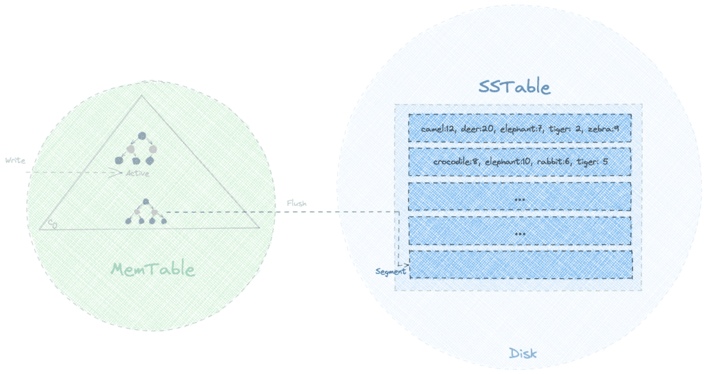
SSTable is the on-disk, immutable format Cassandra uses to persist data. When a MemTable fills up, it’s flushed to disk as an SSTable. Since the flush is a sequential write, it’s fast and is limited mostly by the disk speed.

SSTables aren’t updated in place. Instead, Cassandra periodically compacts multiple SSTables into fewer, larger ones. This background process reorganizes data, removes duplicates, and helps reduce read amplification. The cost of compaction is justified by significantly faster reads down the line.

The SSTable representation. Source: cassandra-storage-engine

Each SSTable consists of three key components:

• Bloom filter for efficient existence checks,
• Index file that maps keys to positions, and
• Data file containing the actual values.

Together, they ensure high write throughput without compromising read performance.

Bloom Filter

Cassandra uses Bloom filters as a first line of defense to avoid unnecessary disk I/O during read operations. These are in-memory, space-efficient, probabilistic data structures that help determine whether a specific row might exist in a particular SSTable. If the Bloom filter says the row doesn’t exist, Cassandra can confidently skip reading that SSTable altogether. This becomes especially important when a node has hundreds or thousands of SSTables after multiple flushes and compactions.

Bloom filters can return false positives. But they never return false negatives.

Bloom filter used to take decisions for data locations. Source: cassandra-storage-engine

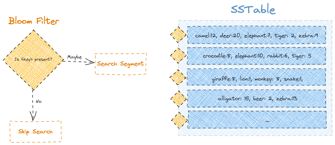
They may indicate that a row might be present even when it’s not. So if a Bloom filter says a row is absent, it’s guaranteed to be true. This allows Cassandra to aggressively reduce disk lookups during reads, especially for sparse or wide-partition workloads where the partition key distribution is uneven.

Index Files

Each SSTable comes with a partition level primary index file, which stores a mapping of partition keys to their corresponding data offsets in the SSTable‘s data file. This index acts as a secondary line of filtering after Bloom filters. It allows Cassandra to quickly perform a binary search to find where in the SSTable a particular row might exist, narrowing down the read scope.

The index is sparse, it doesn’t record every key or column.

Sparse index files used by Cassandra. Source: cassandra-storage-engine

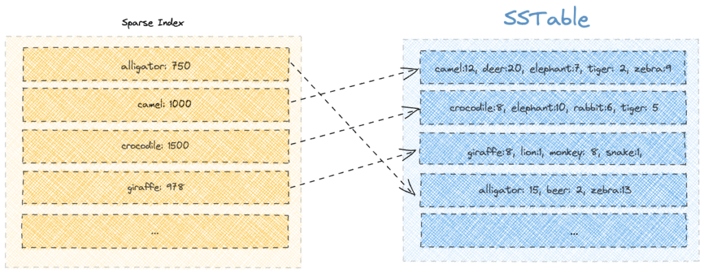
But it’s good enough to locate the nearest block of data on disk. Cassandra loads parts of this index into memory depending on usage and available resources, making access faster for hot partitions. By combining the Bloom filter and the index, Cassandra ensures it only touches disk when there’s a high probability that relevant data exists.

Data Files

Data files (also called Data.db files in the SSTable structure) are where the actual row and column data resides. This is the final destination Cassandra hits during a read operation, only after passing the Bloom filter and index checks.

Data files contain serialized rows, complete with clustering keys, column values, timestamps, and tombstones for deleted data.

Since SSTables are immutable, updates and deletions result in new versions being written to newer SSTables, not overwriting existing data. This design makes writes fast and sequential, but it also means old versions accumulate over time. That’s where compaction later kicks in to merge and reconcile data from multiple SSTables and purge obsolete or deleted information.

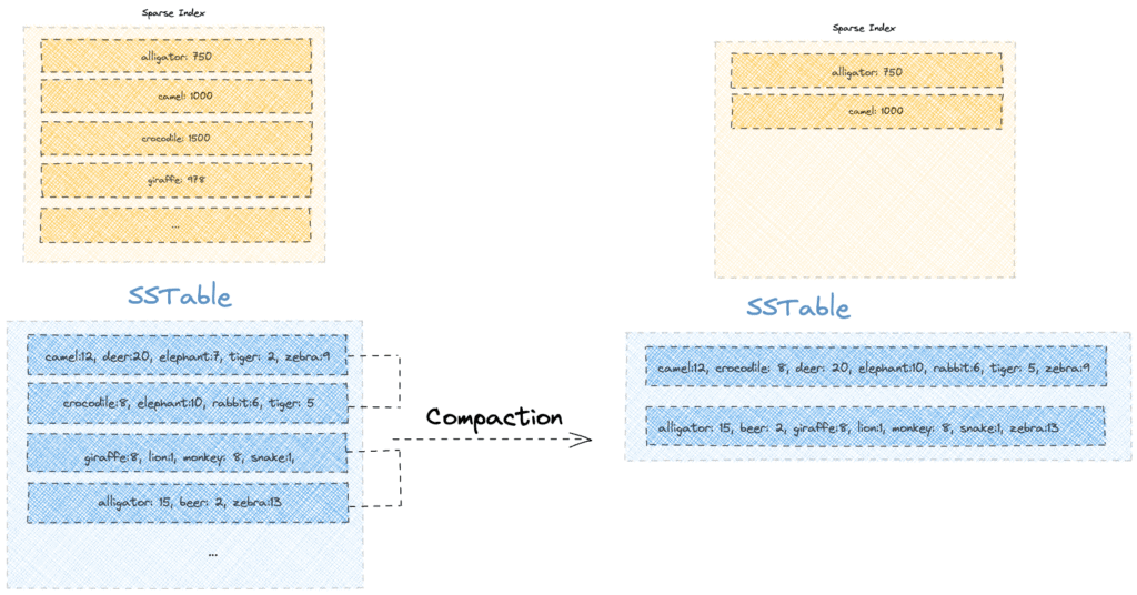
Compaction

A single read in Cassandra might have to scan through multiple SSTables to return a complete result. That means more disk seeks, unnecessary overhead, and even conflict resolution (if the same key exists across files). If left unchecked, this quickly becomes inefficient as SSTables piles up.

To address this, Cassandra uses compaction: a background process that merges multiple SSTables into a single, more organized one. The benefits of compaction are:

• Cleans up tombstones (since Cassandra 0.8+)
• Merges fragmented rows across files
• Rebuilds primary and secondary indexes

Compaction may sound as an extra load, but the merge isn’t as bad as it sounds. SSTables are already sorted, which makes merging more like a streamlined merge-sort than a rewrite-from-scratch.

Cassandra starts by writing SSTables roughly the same size as the MemTable. As these accumulate and the count crosses a configured threshold, the compaction thread kicks in. Typically, four SSTables of equal size are picked and compacted into one larger SSTable.

An important detail here: SSTables selected for compaction are always of similar size.

For example, four 160MB SSTables may produce one ~640MB SSTable. Future compactions in that bucket require other SSTables of similar size, leading to increasing disk usage during merge operations. Bloom filters, partition key indexes, and index summaries are rebuilt in the process to keep read performance optimal.

In effect, every compaction step creates bigger SSTables, leading to more disk space requirements during the merge—but with the long-term benefit of fewer SSTables and faster reads.

Compaction in Action. Source: cassandra-storage-engine

Compaction Strategies

Cassandra supports various compaction strategies. The most common are:

• Size-Tiered Compaction Strategy (STCS): Merges SSTables of similar size once a threshold is reached.
• Leveled Compaction Strategy (LCS): Organizes SSTables into levels with constrained sizes and minimal overlap.

Implementation Details

Cassandra flushes MemTables to disk as SSTables, each approximately the size of the MemTable. Once the number of SSTables in a size tier exceeds the min_threshold (default: 4), Size-Tiered Compaction Strategy (STCS) triggers. The CompactionManager selects SSTables of similar size from the same bucket and performs a k-way merge using iterators over sorted partitions.

During compaction:

• Columns are merged by timestamp for conflict resolution.
• Expired tombstones and deleted data are purged (gc_grace_seconds applies).
• A new SSTable is written using SSTableWriter, and the old ones are atomically replaced.

The key java classes involved are:

• SizeTieredCompactionStrategy.java: Handles size-tier logic.
• CompactionTask.java: Executes the compaction process.
• CompactionManager.java: Schedules background compaction.
• SSTableReader.java / SSTableWriter.java: Reads/writes SSTables.
• CompactionController.java: Manages tombstone handling and merge logic.

Tombstones

We’ve seen how Cassandra writes and stores data for client reads via its nodes. But what happens when we want to delete data?

In Cassandra, even a seemingly simple delete operation needs to be carefully orchestrated. With data flowing through CommitLogs, MemTables, SSTables, and across replicas, deletion must be handled with precision to maintain consistency and correctness.

So, like everything else in Cassandra, deletion is going to be eventful. Deletion, to an extent, follows an update pattern except Cassandra tags the deleted data with a special value, and marks it as a tombstone. This marker helps future queries, compaction, and conflict resolution.

Let’s walk through what happens when a column is deleted.

Deletion of Data

• A client connects to any node (called the coordinator), which might or might not own the data being deleted.
• The client issues a DELETE for column C in column family CF, along with a timestamp.
• If the consistency level is met, the coordinator forwards the delete request to the relevant replica nodes.
• On a replica that holds the row key:
  • The column is either inserted or updated in the MemTable.
  • The value is set to a tombstone—essentially a special marker with:
    • The same column name.
    • A value set to UNIX epoch.
    • The timestamp passed from the client.
• When the MemTable flushes to disk, the tombstone is written to the SSTable like a regular column.

Reading Tombstone Data

• Reads may encounter multiple versions of the same column across SSTables.
• Cassandra reconciles the versions based on timestamps.
  • If the latest value is a tombstone, it’s considered the “correct” one.
• Tombstones are included in the read result internally.
  • But before returning to the client, Cassandra filters out tombstones, so the client never sees deleted data.

Reading Tombstones and Consistency Levels

• For CL > 1, the read is sent to multiple replicas:
  • One node returns the full data.
  • The others return digests (hashes).
• If the digests mismatch (e.g., tombstone not present on some replicas), Cassandra triggers a read repair:
  • The reconciled version (including tombstone) is sent to all involved replicas to ensure consistency.

Compaction and Tombstones

• Tombstones are not removed immediately.
• They’re retained until GCGraceSeconds (default: 10 days) is over.
• During compaction:
  • If the tombstone’s grace period has passed and there’s no conflicting live data, the tombstone is purged.
  • Until then, the tombstone remains to protect against resurrection.

Resurrection Risk

• Suppose a node is down during deletion and stays down past GCGraceSeconds.
• Other replicas delete the data and drop the tombstone during compaction.
• When the downed node comes back:
  • It still holds the original (now-deleted) data.
  • Since no tombstone exists elsewhere, the node assumes it missed a write.
  • It pushes this old data back to the cluster.
• This is called resurrection, and deleted data may reappear in client queries.

Watch Out!

• Always bring downed nodes back within GCGraceSeconds.
• If not, decommission or repair them before bringing them back.
• Regular repairs are crucial to prevent resurrection scenarios in production.

Wrap Up

In the end, Cassandra’s storage engine is all about balance.

It is designed to handle high-speed writes, scale effortlessly, and keep data flowing smoothly even at massive volumes. From memtables and SSTables to compaction, everything works together to support fast, reliable performance. It may seem complex under the hood, but that complexity is what makes Cassandra so powerful in real-world, high-demand environments. Hopefully, this gave you a clearer view of how it all fits together and why Cassandra’s storage engine is one of its biggest strengths.

Stay healthy, stay blessed!